 This is an attempt to offer a somewhat intuitive explanation of why
Simpson's rule is exact for cubic polynomials even though it only
uses quadratic polynomials to approximate the integrand function.
Recall
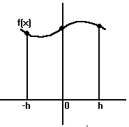
that in each interval (xj, xj+2), Simpson's rule
constructs a quadratic polynomial that agrees with the function being
integrated at the points [xj, f(xj)],
[xj+1, f(xj+1)], and
[xj+2, f(xj+2)]. (See figure)
This is an attempt to offer a somewhat intuitive explanation of why
Simpson's rule is exact for cubic polynomials even though it only
uses quadratic polynomials to approximate the integrand function.
Recall
that in each interval (xj, xj+2), Simpson's rule
constructs a quadratic polynomial that agrees with the function being
integrated at the points [xj, f(xj)],
[xj+1, f(xj+1)], and
[xj+2, f(xj+2)]. (See figure)
 make this discussion easier, we can translate the y-axis so that
it passes through the point xj+1 without changing the
shape of the curves involved, the width of the intervals, or the
results of any of the computations.
Since Simpson's rule uses equally spaced intervals, we can now label
the point that was originally xj+1 as 0 and then label
xj as -h and xj+2 as +h as shown. Now the
cubic polynomial f(x) has the general form
ax3+bx2+cx+d, and the quadratic polynomial
generated by Simpson's rule has the general form
ex2+fx+g. The error function then is
E(x)=ax3+bx2+cx+d-(ex2+fx+g) which
has the general form px3+qx2+rx+s, and the
integral of E(x) from -h to h is the error in the Simpson method within
this interval. Now since the quadratic polynomial agrees with f(x)
at the endpoints and midpoints, we have E(-h)=E(0)=E(h)=0. Evaluating
E(0) we have s=0, so E(x) actually has the form px3+qx2+rx
Evaluating E(-h) and E(h), we get:
make this discussion easier, we can translate the y-axis so that
it passes through the point xj+1 without changing the
shape of the curves involved, the width of the intervals, or the
results of any of the computations.
Since Simpson's rule uses equally spaced intervals, we can now label
the point that was originally xj+1 as 0 and then label
xj as -h and xj+2 as +h as shown. Now the
cubic polynomial f(x) has the general form
ax3+bx2+cx+d, and the quadratic polynomial
generated by Simpson's rule has the general form
ex2+fx+g. The error function then is
E(x)=ax3+bx2+cx+d-(ex2+fx+g) which
has the general form px3+qx2+rx+s, and the
integral of E(x) from -h to h is the error in the Simpson method within
this interval. Now since the quadratic polynomial agrees with f(x)
at the endpoints and midpoints, we have E(-h)=E(0)=E(h)=0. Evaluating
E(0) we have s=0, so E(x) actually has the form px3+qx2+rx
Evaluating E(-h) and E(h), we get:E(-h)=-ph3+qh2-rh=0
E(h)=ph3+qh2+rh=0 and adding these two equations together gives
2qh2=0
Since h is not zero, we must have q=0, so E(x) has the form E(h)=px3+rx
But this means E(x) is an odd function [that is, E(-x)=-E(x), so E(x) is symmetric about the origin], and therefore